Multivariate Regression(WIP):
When it comes to multivariate we will resort to sklearns Polyfeatures() along with Pipeline(). This will facilitate for a more readable code.
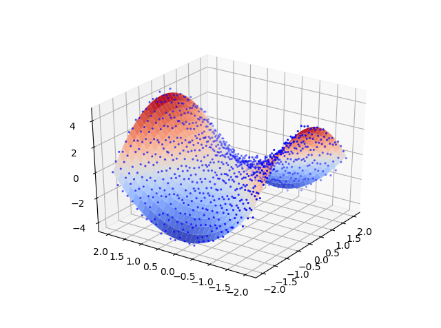
The steps are very similar to the previous example. The only difference is that we will create function of [x,y] and evaluate it in order to create some dummy data. Then the data is fed through a pipeline that generate the polynomial features and get the score for the k-folds.
This file contains hidden or bidirectional Unicode text that may be interpreted or compiled differently than what appears below. To review, open the file in an editor that reveals hidden Unicode characters.
Learn more about bidirectional Unicode characters
| import numpy as np | |
| from sklearn.linear_model import LinearRegression | |
| import matplotlib.pyplot as plt | |
| from sklearn.model_selection import train_test_split | |
| from sklearn.model_selection import KFold | |
| from sklearn.pipeline import Pipeline | |
| def gaussian_noise(mu,sigma,n): | |
| return np.random.normal(mu,sigma,n) | |
| from sklearn.preprocessing import PolynomialFeatures | |
| degree=8 | |
| mean=0 | |
| sigma=.2 | |
| n=30 | |
| x = np.linspace(-2,2,n) | |
| y = np.linspace(-2,2,n) | |
| X, Y = np.meshgrid(x, y) # create a meshgrid to evaluate z(x,y) | |
| Z=Y**2 – X**2 # evaluate z | |
| # reshape for sklearn and add noise | |
| Z=Z.reshape(1,-1).T+np.array([gaussian_noise(mean,sigma,n**2)]).T | |
| X=X.reshape(1,-1).T | |
| Y=Y.reshape(1,-1).T | |
| # input features shape [2,n**2] n= len(x) or len(y) | |
| data=np.concatenate([X,Y],axis=1) | |
| # split to test train sets | |
| _x,x_test,_y,y_test = train_test_split(data, Z,\ | |
| test_size=0.30, | |
| random_state=1337) | |
| # create expression for pipline | |
| estimators=lambda x:[('PolyFeatures',PolynomialFeatures(degree=x)),\ | |
| ('clf',LinearRegression())] | |
| # create a pipeline for every order of poly. | |
| models=[Pipeline(estimators(m)) for m in range(degree)] | |
| # create a generator for 10 folds | |
| kf=KFold(10) | |
| valid_error=[] # variable to store the valid error | |
| train_error=[] # variable to store the train error | |
| for m in models: | |
| # function: fit and get r2 score of model. | |
| f=lambda t,v:m.fit(_x[t],_y[t]).\ | |
| score(_x[v],_y[v]) | |
| # validation scores for each fold | |
| v_score=[f(train,valid) for valid,train in kf.split(_x)] | |
| # training score for each fold | |
| t_score=[f(train,train) for _,train in kf.split(_x)] | |
| # average valid and test error for all folds | |
| valid_error.append(1-sum(v_score)/len(v_score)) | |
| train_error.append(1-sum(t_score)/len(t_score)) | |
| k=np.argmin(valid_error) | |
| # fit model to training and validation data | |
| models[k].fit(_x[:,0:k+1],_y) | |
| # score model against testing data | |
| k_score=models[k].score(x_test[:,0:k+1],y_test) | |
| print('Optimum polynomial order = {0}\n\ | |
| testing score = {1:.2f}'.format(k,k_score)) | |
| #plotting | |
| fig = plt.figure() | |
| ax = fig.gca(projection='3d') | |
| ax.scatter3D(X, Y, Z,linewidth=0, antialiased=True,marker='.',\ | |
| color='blue',label='original data') | |
| X_p, Y_p = np.meshgrid(x, y) | |
| Z_p=models[k].predict(data).reshape(n,n) | |
| from matplotlib import cm | |
| ax.plot_surface(X_p,Y_p,Z_p,cmap=cm.coolwarm,linewidth=0,\ | |
| antialiased=True,label='Predicted Surface') | |
| fig2,ax2=plt.subplots() | |
| ax2.set_xlabel('Polynomial Order'),ax2.set_ylabel('Error') | |
| ax2.plot(train_error,label='Train Error') | |
| ax2.plot(valid_error,label='Valid Error') | |
| ax2.grid(),ax2.legend() |
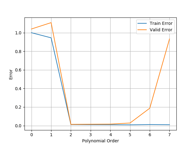
As you can see the order of the polynomial is (2) as it was set in the code before adding gaussian noise. this concludes this series about polynomial regression.
Github repository :
https://github.com/b00033811/ml-uae
