K-fold Cross-validation for tuning hyper parameters:
The goal of this section is to tune our hyper parameter using a simple grid search; before doing so, observe the effect of fitting a high order polynomial to our data.
As you may have noticed, the higher the order of the polynomial, the more we fit our curve to the training set; notice that at same time our testing score will become low. We are over-fitting to the training data and diverging from the testing data. Intuitively we can deduce that we need to find a polynomial function with an order that performs well on both testing and training sets.
However, by doing so we are inadvertently training on the testing set as well. because we are tuning the hyper parameter based on our testing performance (this will result in bad generalization when new data is introduced).
The solution is to create a validation set that falls between the training and testing sets. We can use this validation set to tune our hyper parameter.
I’ve taken the liberty to convert our polynomial function into a class as shown below to make things neat.
This file contains hidden or bidirectional Unicode text that may be interpreted or compiled differently than what appears below. To review, open the file in an editor that reveals hidden Unicode characters.
Learn more about bidirectional Unicode characters
| """ | |
| Polynomial Class | |
| @author: Abdullah Alnuaimi | |
| """ | |
| class Poly(): | |
| def __init__(self,a,k): | |
| self.a=a | |
| self.k=k | |
| self.A =lambda x,a=a,k=k:[[a*n**k for a,k in zip(a,k)] for n in x] | |
| self.V=None | |
| def fit(self,x): | |
| self.V=self.A(x) | |
| def evaluate(self): | |
| assert self.V != None, "No data to evaluate, please fit\ | |
| data using the poly.fit() method" | |
| return [sum(i) for i in self.V] | |
| def poly_features(self): | |
| assert self.V != None, "No data to generate matrix, please fit\ | |
| data using the poly.fit() method" | |
| return self.V |
Since we are doing K-fold cross-validation. the validation set consists of K-folds, where each fold is split into a training/validation set. Each of the folds is passed on to our model. The result of passing all of the folds is averaged into a single value that represents the performance of our model.
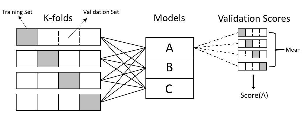
In this case this case the number of models corresponds to the highest order polynomial of our choice.
This file contains hidden or bidirectional Unicode text that may be interpreted or compiled differently than what appears below. To review, open the file in an editor that reveals hidden Unicode characters.
Learn more about bidirectional Unicode characters
| import numpy as np | |
| from sklearn.linear_model import LinearRegression | |
| import matplotlib.pyplot as plt | |
| from sklearn.model_selection import train_test_split | |
| from Poly import Poly | |
| from sklearn.model_selection import KFold | |
| #%% Import Data | |
| x_raw,y_raw=np.loadtxt('data.csv',delimiter=',') | |
| # k = 8 | |
| degree=8 # k=8 | |
| # Initialize the polynomial class and fit | |
| p0=Poly([1]*(degree+1),list(range(0,degree+1))) | |
| p0.fit(x_raw) | |
| # Get the polynomial features for 8th order model | |
| poly_features=p0.poly_features() | |
| # reshape the data | |
| x=np.array(poly_features) | |
| y=y_raw.reshape(-1,1) | |
| # split the model into test/train sets | |
| _x,x_test,_y,y_test=train_test_split(x,y,test_size=.3, | |
| random_state=1337, | |
| shuffle=True) | |
| #%% Split into Kfold and get the test/valid score. | |
| # Create 4 folds | |
| folds=4 | |
| kf=KFold(folds) | |
| # Initiate classifiers | |
| models=[LinearRegression() for m in range(0,degree)] | |
| valid_error=[] # variable to store the valid error | |
| train_error=[] # variable to store the train error | |
| #looping on every model. | |
| for k,m in enumerate(models): | |
| # get poly features for current order [k] poly. model | |
| k_features=_x[:,0:k+1] | |
| # function: fit and get r2 score of model. | |
| f=lambda t,v:m.fit(k_features[t],_y[t]).\ | |
| score(k_features[v],_y[v]) | |
| # validation scores for each fold | |
| v_score=[f(train,valid) for valid,train in kf.split(_x)] | |
| # training score for each fold | |
| t_score=[f(train,train) for _,train in kf.split(_x)] | |
| # average valid and test error for all folds | |
| valid_error.append(1-sum(v_score)/len(v_score)) | |
| train_error.append(1-sum(t_score)/len(t_score)) | |
| # get best model poly. order | |
| k=np.argmin(valid_error) | |
| # fit model to training and validation data | |
| models[k].fit(_x[:,0:k+1],_y) | |
| # score model against testing data | |
| k_score=models[k].score(x_test[:,0:k+1],y_test) | |
| print('Optimum polynomial order = {0}\n\ | |
| testing score = {1:.2f}'.format(k,k_score)) | |
| #%% plotting | |
| fig1,ax=plt.subplots() | |
| ax.set_xlabel('x'),ax.set_ylabel('f(x)') | |
| y_pred=models[k].predict(x[:,0:k+1]) | |
| ax.plot(x_raw,y_pred,color='b',\ | |
| label='Polynomial model k={1} | R2={0:.2f}'.format(k_score,k)) | |
| ax.scatter(x_raw,y_raw,color='r',marker='.',label='Input data') | |
| ax.grid(),ax.legend() | |
| fig2,ax2=plt.subplots() | |
| ax2.set_xlabel('Polynomial Order'),ax2.set_ylabel('Error') | |
| ax2.plot(train_error,label='Train Error') | |
| ax2.plot(valid_error,label='Valid Error') | |
| ax2.grid(),ax2.legend() |
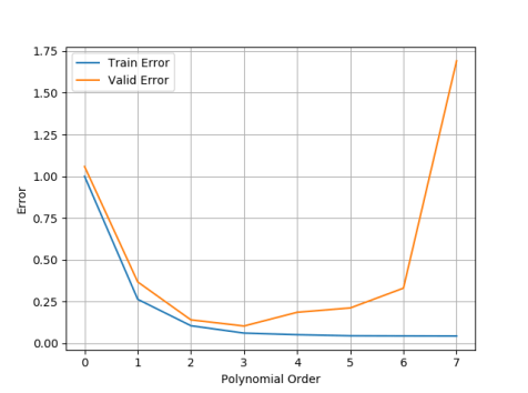
As see you can deduce from the output; the point were the validation error reaches a minimum corresponds with the ideal polynomial order. Furthermore the effect of overfitting is apparent as the polynomial order increases.
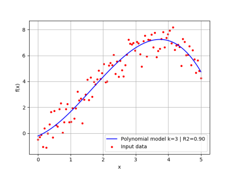
The result of fitting a 3rd order polynomial is identical as the last section.
We are going to end our discussion of Linear Regression with a multivariate example in the next page.
