The focus of this article is to illustrate the application of linear regression using the sklearn library in python. Work in progress (5/30/2018)
Overview:
1. Polynomials in Python.
2. Generating sample data.
3. Fit a linear regressor and evaluate the R2 score.
4. Polynomial Regression.
5. K-Fold cross-validation.
6. Multivariate Regression.
Polynomials in Python:
Before delving into linear regression, let us create a function that evaluates polynomials using the matrix form of a polynomial.
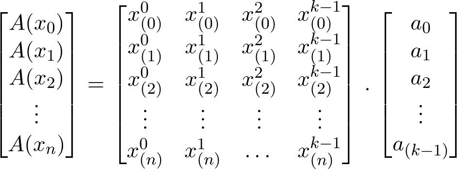
Notice that each row represents a single data point; the row is passed through by taking the dot product of the Vandermonde matrix and the coefficient matrix. The result of the first dot product is:
![]()
A0 is the linear combination of all the terms in the polynomial evaluated at x0. Using this method we can evaluate a polynomial by passing a list of values x:[n_points] where the result of every value in the list is mapped out as the following:
![]()
we can code this up in python with a couple of lines of code.
This file contains hidden or bidirectional Unicode text that may be interpreted or compiled differently than what appears below. To review, open the file in an editor that reveals hidden Unicode characters.
Learn more about bidirectional Unicode characters
| """ | |
| Polynomials | |
| @author: Abdullah Alnuaimi | |
| """ | |
| import numpy as np | |
| import matplotlib.pyplot as plt | |
| def fit_poly(a,k): | |
| '''returns a function of the dot product (A=V.a) ''' | |
| A=lambda x,a=a,k=k:[[a*n**k for a,k in zip(a,k)] for n in x] | |
| return A | |
| def evaluate_poly(x,A): | |
| ''' evaluates A=V.a,stores it in matrix form, and | |
| returns a list y(x)=[A0,..An]''' | |
| y=[sum(i) for i in A(x)] | |
| return y,A(x) | |
| ############################## Main ######################################### | |
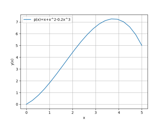
| # y(x)=x+x^2-0.2x^3 | |
| coefficients=[0,1,1,-.2] # polynomial | |
| degree=[0,1,2,3] | |
| A=fit_poly(coefficients,degree) # returns A(x0)…A(Xn) | |
| # Evaluate the functions and returns y(x) | |
| x=np.linspace(0,5,20) | |
| y,_=evaluate_poly(x,A) | |
| #Plotting | |
| plt.plot(x,y,label='p(x)=x+x^2-0.2x^3') | |
| plt.xlabel('x') | |
| plt.ylabel('y(x)') | |
| plt.legend() | |
| plt.grid() |
Now whenever we need to create a polynomial function all we have to do is specify the coefficients and the order of the polynomial.
I should add the calling the function fit_poly() instantiates A(x) however it’s evaluated once evalute_poly() is called and fed with input data. This adds some flexibility without creating classes.
(which we just might…)
