Naive Bayes:
The Naive Bayes classifier assumes independence and that the likelihood of the data can be described as a gaussian function.

where:

If we only care about classification, then we can drop the normalizing factor P(x) and find the argmax of the equation. We will end up with something called the maximum a posteriori (MAP)
![]()
In many cases, there will not be any information on the prior as well. If we assume it is uniform and remove it from the equation. we will end up with the maximum likelihood.
![]()
Now let’s assume our data contains N number of x points. Since we assumed independence; the joint probability is simply the product.

Finally let’s take the log of the likelihood and simplify.

If the variance was equal across all classes then you could drop the log(sigma) and the denominator of the last term. We end up with something very familiar, Minimizing the sum of squared errors!
![]()
So the algorithm works by finding the squared error of every data point from the mean of each classes. The class with the minimum distance scores higher and the data point is labeled accordingly.
So all we need to do is find the mean and the variance of every class in our training data!
Python Implementation:
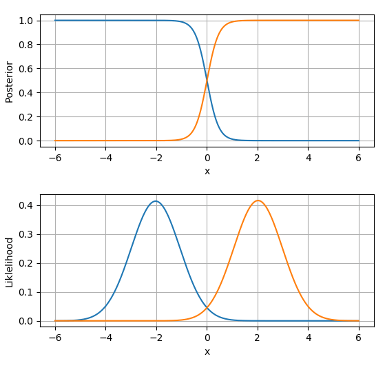
I wrote this python implementation and also calculated the likelihood / evidence and the posterior; just for visualization. The discriminant function is called using the predict method.
I’d like to further note that all values are returned in Log probabilities except the posterior.
This file contains hidden or bidirectional Unicode text that may be interpreted or compiled differently than what appears below. To review, open the file in an editor that reveals hidden Unicode characters.
Learn more about bidirectional Unicode characters
| """ | |
| Univariate Naive Bayes | |
| @author: Abdullah Al Nuaimi | |
| """ | |
| import numpy as np | |
| from scipy.misc import logsumexp | |
| class NB(): | |
| def __init__(self,x,r): | |
| # define the input data | |
| self.x=x | |
| self.r=r | |
| # define the number of data points (t) and hypotheses (i) | |
| self.t,self.i=x.shape[0],r.shape[1] | |
| # initialize a hypotheses set with 2 parameters mean and var | |
| self.H=np.empty((self.i,3)) | |
| def fit(self): | |
| # find the mean,var,prior and store them in hypothesis class (H) | |
| for i in range(0,self.i): | |
| mean=np.average(self.x[self.r[:,i]==1]) | |
| var=np.var(self.x[self.r[:,i]==1],ddof=True) | |
| prior=sum(self.r[:,i]==1)/len(self.r[:,i]) | |
| self.H[i,:]=np.array([mean,var,np.log(prior)]) | |
| return self.H | |
| def likelihood(self,x): | |
| ''' calculate the likelihood of data over all H''' | |
| L=np.empty((len(x),self.i)) | |
| for idx,h in enumerate(self.H): | |
| u=h[0] | |
| v=h[1] | |
| l=(-1/2)*np.log(2*np.pi)-np.log(v)-((x-u)**2/(2*v**2)) | |
| L[:,idx]=l | |
| return L | |
| def evidence(self,x): | |
| MAP=self.likelihood(x)+self.H[:,2] | |
| # e=np.array([np.logaddexp(a,b) for a,b in MAP]) | |
| e=logsumexp(MAP,axis=1) | |
| return e | |
| def posterior(self,x): | |
| return np.exp((self.likelihood(x)+self.H[:,2])-self.evidence(x)[:,None]) | |
| def predict(self,x): | |
| g= -(-np.log(self.H[:,1])-self.H[:,0]+x[:,None])**2/(2*self.H[:,1]**2) | |
| return np.eye(self.i)[np.argmax(g,axis=1)] |
To run this class use the following code
This file contains hidden or bidirectional Unicode text that may be interpreted or compiled differently than what appears below. To review, open the file in an editor that reveals hidden Unicode characters.
Learn more about bidirectional Unicode characters
| # -*- coding: utf-8 -*- | |
| """ | |
| Created on Sun Jun 24 00:26:00 2018 | |
| @author: b0003 | |
| """ | |
| import numpy as np | |
| np.random.seed(1337) | |
| from NaiveBayes_log import NB | |
| import matplotlib.pyplot as plt | |
| from sklearn.preprocessing import OneHotEncoder | |
| def data_gen(param,n,shuffle='False'): | |
| data=np.empty((0,2)) | |
| for u,v,l in param: | |
| x=np.random.normal(u,v,n).reshape(n,1) | |
| y=np.full((n,1),l) | |
| data=np.append(data,np.concatenate([x,y],axis=1),axis=0) | |
| if shuffle=='True': | |
| np.random.shuffle(data) | |
| return data | |
| return data | |
| param=[[-2,1,0],[2,1,1]] | |
| raw_data=data_gen(param,1000,shuffle='True') | |
| x=raw_data[:,0] | |
| r=raw_data[:,1].reshape(-1,1) | |
| encoder=OneHotEncoder() | |
| r=encoder.fit_transform(r).toarray() | |
| model=NB(x,r) | |
| H=model.fit() | |
| x=np.linspace(-6,6,1000) | |
| p=model.posterior(x) | |
| l=model.likelihood(x) | |
| fig,ax=plt.subplots(2,1) | |
| for axs in ax: | |
| axs.grid() | |
| ax[0].plot(x,p) | |
| ax[0].set_xlabel('x') | |
| ax[0].set_ylabel('Posterior') | |
| ax[1].plot(x,np.exp(l)) | |
| ax[1].set_xlabel('x') | |
| ax[1].set_ylabel('Liklelihood') | |
| plt.show() | |
| plt.tight_layout() |
I hope this demonstrates how easy it is to implement Naive Bayes in code. The next step would be to move on into multivariate NB.
Again all files can be found at http://github.com/b00033811/ml-uae
